LTspice with Python 1. rawファイル読み込み

LTspiceの電気回路シミュレータをPythonで利用する方法を紹介する
今回は、LTspiceで実行したシミュレーション結果(rawファイル)を読み込んで可視化する

LTspice with Python 1. rawファイル読み込み

回路図作成

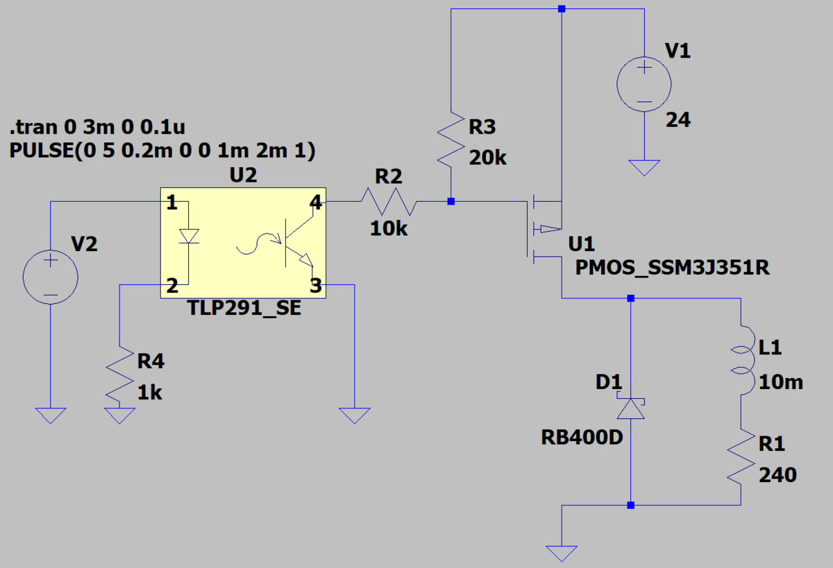
PチャネルMOSFET (SSM3J351R) を使って、圧空系の電磁弁を駆動する回路を作成する

ロジック側(5VD)とドライブ側(24VL)との分離のため、フォトカプラを間に使用する
PチャネルMOSFETを使用して、電磁弁をソース駆動させる
電磁弁のインダクタンスによる逆起電圧の防止用にダイオードを追加する

シミュレーション結果(rawファイル)の可視化

rawファイルの読み込み

ファイルを読み込み、基本的な情報を確認する
作成した回路図でシミュレーションを実行して、rawファイルを生成しておく

import matplotlib.pyplot as plt
from PyLTSpice import RawRead

LTR = RawRead("P-MOSFET.raw")
print(LTR.get_trace_names())

['time', 'V(n006)', 'V(n001)', 'V(n004)', 'V(n007)', 'V(n003)', 'V(n002)', 'V(n005)', 'I(D1)', 'I(L1)', 'I(R4)', 'I(R3)', 'I(R2)', 'I(R1)', 'I(V2)', 'I(V1)', 'Ix(u1:1)', 'Ix(u1:2)', 'Ix(u1:3)', 'Ix(u2:1)', 'Ix(u2:2)', 'Ix(u2:3)', 'Ix(u2:4)']

LTR_info = LTR.get_raw_property()
for key in LTR_info.keys():
    print(key, ':', LTR_info[key])

Filename : P-MOSFET.raw
Title : * C:\Users\XXXX\LTspice\P-MOSFET\P-MOSFET.asc
Date : XXXX
Plotname : Transient Analysis
Flags : real forward
No. Variables : 23
No. Points : 836
Offset : 0.0000000000000000e+000
Command : Linear Technology Corporation LTspice XVII
Backannotation : u2 1 2 3 4
Variables : ['time', 'V(n006)', 'V(n001)', 'V(n004)', 'V(n007)', 'V(n003)', 'V(n002)', 'V(n005)', 'I(D1)', 'I(L1)', 'I(R4)', 'I(R3)', 'I(R2)', 'I(R1)', 'I(V2)', 'I(V1)', 'Ix(u1:1)', 'Ix(u1:2)', 'Ix(u1:3)', 'Ix(u2:1)', 'Ix(u2:2)', 'Ix(u2:3)', 'Ix(u2:4)']

複数のシミュレーション条件がある場合は、steps = LTR.get_steps() で情報を取得できる

可視化

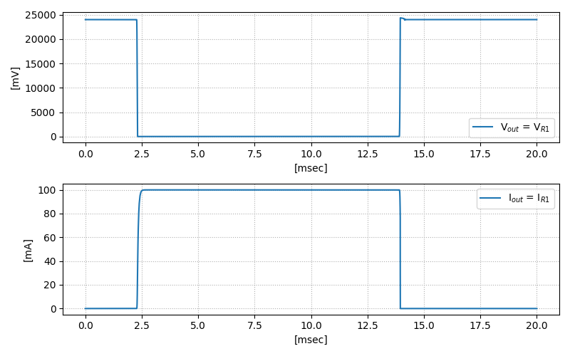
電磁弁への出力電圧、電流
フォトカプラの入力電圧、電流
FETのゲート電圧

fig = plt.figure(figsize=(10, 4))

time = LTR.get_trace('time')
step = 0

ax1 = fig.add_subplot(2, 3, 1)
Vn006 = LTR.get_trace("V(n006)")
ax1.plot(time.get_wave(step) * 1e3, Vn006.get_wave(step), label='V$_{out}$ = V$_{R1}$')
ax1.set_xlabel('[msec]'); ax1.set_ylabel('[V]')
ax1.legend()
ax1.grid(which='both', ls=':')

ax2 = fig.add_subplot(2, 3, 4, sharex=ax1)
IR1   = LTR.get_trace("I(R1)")
ax2.plot(time.get_wave(step) * 1e3, IR1.get_wave(step) * 1e3, label='I$_{out}$ = I$_{R1}$')
ax2.set_xlabel('[msec]'); ax2.set_ylabel('[mA]')
ax2.legend()
ax2.grid(which='both', ls=':')

ax3 = fig.add_subplot(2, 3, 2, sharex=ax1)
Vn002 = LTR.get_trace("V(n002)")
ax3.plot(time.get_wave(step) * 1e3, Vn002.get_wave(step), label='V$_{in}$')
ax3.set_xlabel('[msec]'); ax3.set_ylabel('[V]')
ax3.legend()
ax3.grid(which='both', ls=':')

ax4 = fig.add_subplot(2, 3, 5, sharex=ax1)
IR4   = LTR.get_trace("I(R4)")
ax4.plot(time.get_wave(step) * 1e3, IR4.get_wave(step) * 1e3, label='I$_{R4}$')
ax4.set_xlabel('[msec]'); ax4.set_ylabel('[mA]')
ax4.legend()
ax4.grid(which='both', ls=':')

ax5 = fig.add_subplot(2, 3, 3, sharex=ax1)
Vn004 = LTR.get_trace("V(n004)")
ax5.plot(time.get_wave(step) * 1e3, Vn004.get_wave(step), label='V$_{Gate}$')
ax5.set_xlabel('[msec]'); ax5.set_ylabel('[V]')
ax5.legend()
ax5.grid(which='both', ls=':')

ax6 = fig.add_subplot(2, 3, 6, sharex=ax1)
IR2   = LTR.get_trace("I(R2)")
ax6.plot(time.get_wave(step) * 1e3, IR2.get_wave(step) * 1e3, label='I$_{R2}$')
ax6.set_xlabel('[msec]'); ax6.set_ylabel('[mA]')
ax6.legend()
ax6.grid(which='both', ls=':')

fig.tight_layout()

出力側
- 24Vが供給され、24V / 240Ω = 100mA が出力
入力側
5Vを入れていて、R4には、フォトカプラ分の1.2Vほど電圧降下により、(5V - 1.2V) / 1kΩ = 3.8mA が流れる
FETのゲート側
- フォトカプラが通電し、24V / (10kΩ + 20kΩ) = 0.8mA が流れる
- 電圧
  - OFF時は、24Vで、GS間の電圧はほぼ0Vで動作しない
  - ON時は、8Vで、GS間の電圧が-16Vになり、動作する

分析 - オン抵抗

MOSFETの場合、ドレイン(D)-ソース(S)間のオン時の抵抗値が重要な性能になる
シミュレーション結果の、MOSFETのDS間の電圧差と電流値からオン抵抗を取得する

fig = plt.figure(figsize=(8, 5))

time = LTR.get_trace('time')
step = 0

ax1 = fig.add_subplot(2, 1, 1)
Vn001 = LTR.get_trace("V(n001)")
Vn006 = LTR.get_trace("V(n006)")
data = Vn001.get_wave(step) - Vn006.get_wave(step)
ax1.plot(time.get_wave(step) * 1e3, data * 1e3, label='V$_{out}$ = V$_{R1}$')
ax1.set_xlabel('[msec]'); ax1.set_ylabel('[mV]')
ax1.legend()
ax1.grid(which='both', ls=':')

ax2 = fig.add_subplot(2, 1, 2, sharex=ax1)
IxS = LTR.get_trace("Ix(U1:3)")
data = IxS.get_wave(step)
ax2.plot(time.get_wave(step) * 1e3, data * 1e3, label='I$_{out}$ = I$_{R1}$')
ax2.set_xlabel('[msec]'); ax2.set_ylabel('[mA]')
ax2.legend()
ax2.grid(which='both', ls=':')

fig.tight_layout()

オン時（t = 4 ~ 12 sec まで）を抽出して、電圧 / 電流で抵抗値を求める

fig = plt.figure(figsize=(9, 5))

time_org = LTR.get_trace('time')
step = 0
t_range = [4.0, 12.0]

IxS = LTR.get_trace("Ix(U1:3)").get_wave(step)
time_org = time_org.get_wave(step) * 1e3
time = time_org[(time_org > t_range[0]) & (time_org < t_range[1])]

Vn001 = LTR.get_trace("V(n001)")
Vn006 = LTR.get_trace("V(n006)")
data = Vn001.get_wave(step) - Vn006.get_wave(step)
data1 = data[(time_org > t_range[0]) & (time_org < t_range[1])]

data2 = IxS[(time_org > t_range[0]) & (time_org < t_range[1])]

data3 = data1 / IxS[(time_org > t_range[0]) & (time_org < t_range[1])]

ax1 = fig.add_subplot(3, 1, 1)
ax1.plot(time, data1 * 1e3, label='V$_{out}$ = V$_{R1}$')
ax1.set_xlabel('[msec]'); ax1.set_ylabel('[mV]')
ax1.legend()
ax1.grid(which='both', ls=':')

ax2 = fig.add_subplot(3, 1, 2, sharex=ax1)
ax2.plot(time, data2 * 1e3, label='I$_{out}$ = I$_{R1}$')
ax2.set_xlabel('[msec]'); ax2.set_ylabel('[mA]')
ax2.legend()
ax2.grid(which='both', ls=':')

ax3 = fig.add_subplot(3, 1, 3, sharex=ax1)
ax3.plot(time, data3 * 1e3, label='R$_{DS}$')
ax3.set_xlabel('[msec]'); ax3.set_ylabel('[mΩ]')
ax3.legend()
ax3.grid(which='both', ls=':')

fig.tight_layout()

print('%7.1fmV %7.1fmA %7.1fmΩ' % (data1.mean() * 1e3, data2.mean() * 1e3, data3.mean() * 1e3))

   11.0mV   100.0mA   110.5mΩ

オン抵抗は、110mΩ程度
カタログスペックでは、最大値で、134mΩ ~ 184mΩ が記載されているので、大体あっている

このオン抵抗によって、100mA流れた場合は、11mVの電圧低下が供給側に発生する
ロード側の許容範囲を確認して問題ないか確認する必要がある

また、MOSFETの消費電力は、11mV x 100mA = 1.1mW になる
許容損失は 1W なので、余裕なことがわかる

私の拙い知識で書いておりますので、誤り等ありましたらご指摘ください