前回 : Pythonによる制御工学入門第4回 - ma-hi-ro Hobby

Pythonによる制御工学入門第5回

今回は、参考書の6章「開ループ系に注目した制御設計」の
6.3「位相進み遅れ補償」のフィルタを自作の数値シミュレーションで再現しつつ、
デジタルフィルタの設計方法を紹介する

Pythonによる制御工学入門第5回

位相進み遅れ補償

下記の垂直駆動アームの設計を行う
ゲイン交差周波数（開ループのゲインが 0[dB] になる周波数）を 40[rad/s]
位相余裕を 60[deg]
とする

g  = 9.81                # 重力加速度[m/s^2]
l  = 0.2                 # アームの長さ[m]
M  = 0.5                 # アームの質量[kg]
mu = 1.5e-2              # 粘性摩擦係数[kg*m^2/s]
J  = 1.0e-2              # 慣性モーメント[kg*m^2]

P = pyctrl.tf([0, 1], [J, mu, M*g*l])

位相遅れ補償

特徴

低域のゲインを上げることができる
ただし、位相が遅れるため、発振しやすくなる
- $\frac{1}{\alpha T_1}$ ～ $\frac{1}{T_1}$ の位相が遅れる
- 悪化量は、最大で、 $\omega_m = \frac{1}{T_1 \sqrt{\alpha}}$ で、 $\phi_m = sin^{-1} \frac{1 - \alpha}{1 + \alpha}$ だけ遅れる

$\displaystyle K_1 (s) = \alpha \frac{T_1 s + 1}{\alpha T_1 s + 1} \space (\alpha > 1)$

設計方法

$T_1$ は、位相が遅れすぎないように、 $\frac{1}{T_1}$ が、目標のゲイン交差周波数の10分の1になるようにする
今回は、 40[rad/s] が目標値なので、 $\frac{1}{T_1}$ = 40 / 10 = 4[rad/s] になるように、 $T_1$ = 0.25 とする

$\alpha$ は、大きい方が低域のゲインが大きくなるが、大きすぎると位相の遅れが大きくなるので、
とりあえず、 $\alpha$ = 20 とする

位相進み補償

特徴

高域のゲインを上げることができる
また、位相を進めて、位相余裕を広げることができる
- $\frac{1}{T_2}$ ～ $\frac{1}{\beta T_2}$ の位相が進む
- 最大で、 $\omega_m = \frac{1}{T_2 \sqrt{\beta}}$ で、 $\phi_m = sin^{-1} \frac{1 - \beta}{1 + \beta}$ だけ進む

$\displaystyle K_2 (s) = \frac{T_2 s + 1}{\beta T_2 s + 1} \space (\beta < 1)$

設計方法

ゲイン交差周波数における位相遅れが設計値 -120[deg] になるようにする
位相が -183.136[deg] の場合は、 +63.136[deg] する必要がある
$\beta = \frac{1 - sin 63.136}{1 + sin 63.136}$ = 0.05703

次に、 $\frac{1}{\beta T_2}$ が 40[rad/s] になるようにする
$T_2 = \frac{1}{40 \sqrt{\beta}}$ = 0.10467

Controlモジュールによる設計シミュレーション

位相遅れ補償の設計

$\displaystyle K_1 = \frac{5 s + 20}{5 s + 1}$

alpha = 20
T1 = 0.25
K1 = pyctrl.tf([alpha * T1, alpha], [alpha * T1, 1])

H1 = P * K1
[mag], [phase], _ = pyctrl.freqresp(H1, [40])
phaseH1at40 = phase * (180/np.pi)
if phaseH1at40 > 0:
    phaseH1at40 -= 360

fig = plt.figure(figsize=(6, 5))
ax1 = fig.add_subplot(2, 1, 1)
ax2 = fig.add_subplot(2, 1, 2)

gain, phase, w = pyctrl.bode(P, pyctrl.logspace(-1,2), plot=False)
ax1.plot(w/(2*np.pi), 20*np.log10(gain), label='P')
ax2.plot(w/(2*np.pi), phase*180/np.pi, label='P')

gain, phase, w = pyctrl.bode(H1, pyctrl.logspace(-1,2), plot=False)
ax1.plot(w/(2*np.pi), 20*np.log10(gain), label='H1')
ax2.plot(w/(2*np.pi), phase*180/np.pi, label='H1')
ax2.plot(40.0/(2*np.pi), phaseH1at40, 'o', label='40rad/s')

ax2.set_ylim(-190, 10); ax2.set_yticks([-180, -90, 0])
ax1.legend(); ax1.grid(which='both'); ax1.set_xscale('log')
ax1.set_ylabel('Gain [dB]')
ax2.legend(); ax2.grid(which='both'); ax2.set_xscale('log')
ax2.set_xlabel('[Hz]')
ax2.set_ylabel('Phase [deg]')
fig.tight_layout()

低域のゲインが上がっている
位相が遅れているので、このままゲインを上げると発振してしまう
位相進み補償で補正する必要がある

位相進み補償の設計

$\displaystyle K_2 = \frac{0.1047 s + 1}{0.005971 s + 1}$

phim = (60- (180 + phaseH1at40)) * np.pi/180
beta = (1 - np.sin(phim)) / (1 + np.sin(phim))
T2 = 1 / 40 / np.sqrt(beta)
K2 = pyctrl.tf([T2, 1],[beta * T2, 1])

H2 = P * K1 * K2
[mag], [phase], _ = pyctrl.freqresp(H2, [40])
magH2at40 = mag
phaseH2at40 = phase * (180/np.pi)

fig = plt.figure(figsize=(6, 5))
ax1 = fig.add_subplot(2, 1, 1)
ax2 = fig.add_subplot(2, 1, 2)

gain, phase, w = pyctrl.bode(H1, pyctrl.logspace(-1,2), plot=False)
ax1.plot(w/(2*np.pi), 20*np.log10(gain), label='H1')
ax2.plot(w/(2*np.pi), phase*180/np.pi, label='H1')

gain, phase, w = pyctrl.bode(H2, pyctrl.logspace(-1,2), plot=False)
ax1.plot(w/(2*np.pi), 20*np.log10(gain), label='H2')
ax1.plot(40.0/(2*np.pi), 20*np.log10(magH2at40), 'o', label='40rad/s')
ax2.plot(w/(2*np.pi), phase*180/np.pi, label='H2')
ax2.plot(40.0/(2*np.pi), phaseH2at40, 'o', label='40rad/s')

ax2.set_ylim(-190, 10); ax2.set_yticks([-180, -90, 0])
ax1.legend(); ax1.grid(which='both'); ax1.set_xscale('log')
ax1.set_ylabel('Gain [dB]')
ax2.legend(); ax2.grid(which='both'); ax2.set_xscale('log')
ax2.set_xlabel('[Hz]')
ax2.set_ylabel('Phase [deg]')
fig.tight_layout()

位相進み補償により、 40[rad/s] での位相が -120[deg] となっている
あとは、ゲイン補償により、 40[rad/s] のゲインを 0[dB] にすればよい

ゲイン補償の設計

40[rad/s] におけるゲインが -11.06[dB] 程度なので、
ゲイン補償は $k = 1/magL2at40 = 3.57$ とする

k = 1 / magH2at40

H = P * k * K1 * K2

fig = plt.figure(figsize=(6, 5))
ax1 = fig.add_subplot(2, 1, 1)
ax2 = fig.add_subplot(2, 1, 2)

gain, phase, w = pyctrl.bode(H, pyctrl.logspace(-1,2), plot=False)
ax1.plot(w/(2*np.pi), 20*np.log10(gain), label='H')
ax2.plot(w/(2*np.pi), phase*180/np.pi, label='H')

gain, phase, w = pyctrl.bode(P, pyctrl.logspace(-1,2), plot=False)
ax1.plot(w/(2*np.pi), 20*np.log10(gain), label='P')
ax2.plot(w/(2*np.pi), phase*180/np.pi, label='P')

ax2.set_ylim(-190, 10); ax2.set_yticks([-180, -90, 0])
ax1.legend(); ax1.grid(which='both'); ax1.set_xscale('log')
ax1.set_ylabel('Gain [dB]')
ax2.legend(); ax2.grid(which='both'); ax2.set_xscale('log')
ax2.set_xlabel('[Hz]')
ax2.set_ylabel('Phase [deg]')
fig.tight_layout()

40[rad/s] でゲインが 0[dB] と交差し、位相余裕が 60[deg] になっている

数値シミュレーションによる位相進み遅れ補償

前回までと同様に、数値シミュレーションで、再現させる
位相進み遅れ補償をデジタル実装する上では、伝達関数を離散化する必要があり、Z変換を実施する

Z変換

伝達関数の $s$ を離散化の $z$ に変換する
周波数特性を保つため、下記の双一次変換で変換する

$\displaystyle s = \frac{2}{T} \frac{1 - z^{-1}}{1 + z^{-1}}$

遅れ補償、進み補償のフィルタは1次のIIRフィルタになる

フィルタ係数を下記のように表す

$\displaystyle K = \frac{C s + D}{A s + B}$

これに双一次変換を施すと下記になる

$\displaystyle K = \frac{(2 C + D T) - (2 C - D T) z^{-1}}{(2 A + B T) - (2 A - B T) z^{-1}}$

ここで、各項の係数を下記のように表すと

$\displaystyle E = 2 A + B T \\ F = 2 A - B T \\ G = 2 C + D T \\ H = 2 C - D T \\$

$\displaystyle Y = K X = \frac{G - H z^{-1}}{E - F z^{-1}}$

から

$\displaystyle (E - F z^{-1}) Y = (G - H z^{-1}) X$

となる

$z^{-1}$ は 1サンプル前のデータを表すので

$\displaystyle E y_n - F y_{n - 1} = G x_n - H x_{n - 1}$

$\displaystyle y_n = \frac{1}{E} (G x_n - H x_{n - 1} + F y_{n - 1})$

と、入力 $x_n$ から、出力 $y_n$ を求めることができる

フィルタ係数の算出

今回のフィルタ係数からデジタルフィルタの係数を計算する

$\displaystyle K_1 = \frac{5 s + 20}{5 s + 1}$

$\displaystyle K_2 = \frac{0.1047 s + 1}{0.005971 s + 1}$

$\displaystyle k = 3.57$

def calc_EFGH(T, A, B, C, D):
    E = 2 * A + B * T
    F = 2 * A - B * T
    G = 2 * C + D * T
    H = 2 * C - D * T
    return E, F, G, H

def filter(E, F, G, H, x, pre_x, pre_y):
    return (F * pre_y + G * x - H * pre_x) / E

T = 0.001

A1 = 5.0
B1 = 1.0
C1 = 5.0
D1 = 20.0
E1, F1, G1, H1 = calc_EFGH(T, A1, B1, C1, D1)

A2 = 0.005971
B2 = 1.0
C2 = 0.1047
D2 = 1.0
E2, F2, G2, H2 = calc_EFGH(T, A2, B2, C2, D2)

k = 3.57

数値シミュレーションの実施（ステップ応答）

まずは、ステップ応答で、フィルタがControlモジュールの結果と同じになるかを確認する

target = 30.0

dt = 0.001

t_s   = [0.0, dt]
x_s   = [0.0, 0.0]
v_s   = [0.0, 0.0]
a_s   = [0.0, 0.0]
F_s   = [0.0, 0.0]
ref_s = [0.0, 0.0]
err_s = [0.0, 0.0]
y1_s  = [0.0, 0.0]
y2_s  = [0.0, 0.0]

for i in range(2000):
    ref = target
    ref_s += [ref]
    err_s += [ref_s[-1] - x_s[-1]]

    y1_s += [filter(E1, F1, G1, H1, err_s[-1], err_s[-2], y1_s[-1])]
    y2_s += [filter(E2, F2, G2, H2, y1_s[-1],  y1_s[-2],  y2_s[-1])]

    F_s += [y2_s[-1] * k]
    a_s += [(- mu * v_s[-1] - M * g * l * x_s[-1] + F_s[-1]) / J]
    v_s += [v_s[-1] + a_s[-1] * dt]
    x_s += [x_s[-1] + v_s[-1] * dt]
    t_s += [t_s[-1] + dt]

df = pd.DataFrame()
df['in']  = F_s[::10]
df['out'] = x_s[::10]
df.index  = t_s[::10]

fig = plt.figure(figsize=(6, 5))
ax1 = fig.add_subplot(1, 1, 1)

ax1.plot(df.index, df['out'], '.-', label='sim')

y, t = pyctrl.step(pyctrl.feedback(H, 1), np.arange(0, 2, 0.01))
ax1.plot(t, y * target, '-', label='H')

ax1.axhline(target, color="k", linewidth=0.5)
ax1.set_xlim(0, 2); ax1.set_ylim(0, 50)
ax1.legend(); ax1.grid()
ax1.set_ylabel('y'); ax1.set_xlabel('t')
fig.tight_layout()

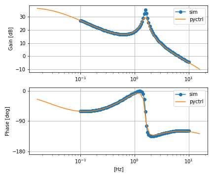
数値シミュレーションの実施（周波数特性）

閉ループ特性を取得して、開ループ特性を算出する

hz_s = []
hz = 0.1
while True:
    if hz > 10 * 10 ** (2 / 100):
        break
    hz_s.append(hz)
    hz = hz * 10 ** (2 / 100)

from scipy.optimize import curve_fit

def sin_func2(x, p0, p1, p2, ofs):
    return p0 * np.sin(2.0 * np.pi * p1 * x + p2) + ofs

def _convert_phase(phase):
    phase += 180
    phase %= 360
    if phase < 0:
        phase += 180
    else:
        phase -= 180
    return phase

def _convert_param(param):
    param = param.copy()
    param[2] = param[2] / np.pi * 180
    if param[0] < 0:
        param[0] = -param[0]
        param[2] += 180

    param[2] = _convert_phase(param[2])

    return param

def calc_f_func(param1, param2):
    param1 = _convert_param(param1)
    param2 = _convert_param(param2)

    freq = param1[1]
    gain = param2[0] / param1[0]
    phase = param2[2] - param1[2]
    phase = _convert_phase(phase)

    return param1, param2, freq, gain, phase

target = 30.0
dt = 0.001
df_list = []
for hz in hz_s:
    t_s   = [0.0, 0.0]
    x_s   = [0.0, 0.0]
    v_s   = [0.0, 0.0]
    a_s   = [0.0, 0.0]
    F_s   = [0.0, 0.0]
    ref_s = [0.0, 0.0]
    err_s = [0.0, 0.0]
    y1_s  = [0.0, 0.0]
    y2_s  = [0.0, 0.0]

    for i in range(50000):
        ref = target * np.sin(2.0 * np.pi * hz * t_s[-1])
        ref_s += [ref]
        err_s += [ref_s[-1] - x_s[-1]]

        y1_s += [filter(E1, F1, G1, H1, err_s[-1],  err_s[-2],  y1_s[-1])]
        y2_s += [filter(E2, F2, G2, H2, y1_s[-1], y1_s[-2], y2_s[-1])]

        F_s += [y2_s[-1] * k]
        a_s += [(- mu * v_s[-1] - M * g * l * x_s[-1] + F_s[-1]) / J]
        v_s += [v_s[-1] + a_s[-1] * dt]
        x_s += [x_s[-1] + v_s[-1] * dt]
        t_s += [t_s[-1] + dt]

    df = pd.DataFrame()
    df['in']  = ref_s[10000:]
    df['out'] = x_s[10000:]
    df.index  = t_s[10000:]
    df_list += [df]

data_s = []
for hz, df in zip(hz_s, df_list):
    p0 = [target, hz, 0.0, df['in'].mean()]
    p1, conv = curve_fit(sin_func2, np.array(df.index), np.array(df['in']), p0=p0)

    p0 = [target, hz, 0.0, df['out'].mean()]
    p2, conv = curve_fit(sin_func2, np.array(df.index), np.array(df['out']), p0=p0)

    param1, param2, freq, gain, phase = calc_f_func(p1, p2)

    data_s.append([freq, gain, phase])

df_res = pd.DataFrame(data_s)
df_res.columns = ['freq', 'gain', 'phase']

gain_open_s = []
phase_open_s = []
for i in df_res.index:
    data = df_res.loc[i]

    tan_theta = np.tan(np.deg2rad(data['phase']))
    A = data['gain'] / np.sqrt(1 + tan_theta**2)
    if abs(data['phase']) > 90:
        A = -A
    B = A * tan_theta

    gain_open  = data['gain'] / np.sqrt(np.abs((1.0 - A)**2 + B**2))
    phase_open = data['phase'] + np.rad2deg(np.arctan2(B, 1 - A))

    gain_open_s  += [gain_open]
    phase_open_s += [phase_open]

df_res['gain_open']  = gain_open_s
df_res['phase_open'] = phase_open_s

fig = plt.figure(figsize=(6, 5))
ax1 = fig.add_subplot(2, 1, 1)
ax2 = fig.add_subplot(2, 1, 2)

ax1.plot(df_res['freq'], np.log10(df_res['gain_open'])*20.0, 'o-', label='sim')
ax2.plot(df_res['freq'], df_res['phase_open'], 'o-', label='sim')

gain, phase, w = pyctrl.bode(H, pyctrl.logspace(-1,2), plot=False)
ax1.plot(w/(2*np.pi), 20*np.log10(gain), label='pyctrl')
ax2.plot(w/(2*np.pi), phase*180/np.pi, label='pyctrl')

ax2.set_ylim(-190, 10); ax2.set_yticks([-180, -90, 0])
ax1.legend(); ax1.grid(); ax1.set_xscale('log')
ax1.set_ylabel('Gain [dB]')
ax2.legend(); ax2.grid(); ax2.set_xscale('log')
ax2.set_xlabel('[Hz]')
ax2.set_ylabel('Phase [deg]')
fig.tight_layout()