LTspice with Python 2. シミュレーションの実行

LTspiceの電気回路シミュレータをPythonで利用する方法を紹介する
今回は、LTspiceで作成した回路図(.asc)を読み込み、Pythonでシミュレーションを実行する

LTspice with Python 2. シミュレーションの実行

回路図作成

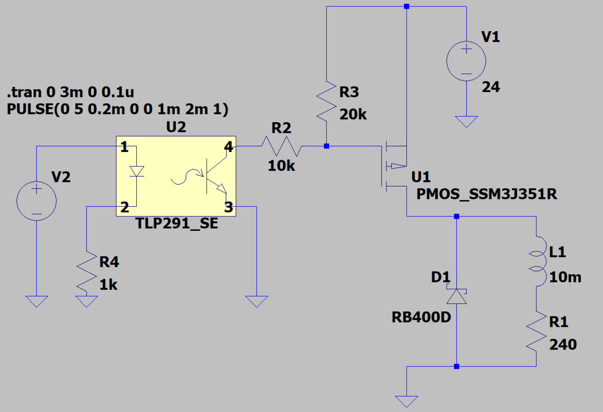
PチャネルMOSFET (SSM3J351R) を使って、圧空系の電磁弁を駆動する回路を作成する

ロジック側(5VD)とドライブ側(24VL)との分離のため、フォトカプラを間に使用する
PチャネルMOSFETを使用して、電磁弁をソース駆動させる
電磁弁のインダクタンスによる逆起電圧の防止用にダイオードを追加する

シミュレーションの実行

ascファイルの読み込み

SimCommander を使って、ascファイルを読み込む
読み込むと同時に、netファイルが生成される

import matplotlib.pyplot as plt
from PyLTSpice import SimCommander

LTC = SimCommander("P-MOSFET.asc")

生成されたnetファイルを確認する

!more P-MOSFET.net

* c:\Users\XXXX\P-MOSFET.asc
L1 N006 N007 10m
R1 N007 0 240
V1 N001 0 24
R2 N004 N003 10k
R3 N001 N004 20k
V2 N002 0 PULSE(0 5 2m 0 0 10m 20m 1)
R4 N005 0 1k
D1 0 N006 RB400D
XU1 N006 N004 N001 PMOS_SSM3J351R
XU2 N002 N005 0 N003 TLP291_SE
.model D D
.lib C:\Users\XXXX\AppData\Local\LTspice\lib\cmp\standard.dio
.tran 0 20m 0 1u
.lib Contrib/Toshiba/LVMOS/SSM3J351R_G0_00.mod
.lib importsub/TLP291_SE.mod
.backanno
.end

このネットリストを元にシミュレーションが実行される

シミュレーションの実行

上記のnetファイルに対して、シミュレーションを実行する

LTC.run('P-MOSFET_tmp.net')
LTC.wait_completion()

シミュレーションが実行され、結果のファイル（P-MOSFET_tmp.raw）が生成される

シミュレーション結果の確認

生成されたrawファイルを可視化する

from PyLTSpice import RawRead
LTR = RawRead("P-MOSFET_tmp.raw")

fig = plt.figure(figsize=(10, 4))

time = LTR.get_trace('time')
step = 0

ax1 = fig.add_subplot(2, 3, 1)
Vn006 = LTR.get_trace("V(n006)")
ax1.plot(time.get_wave(step) * 1e3, Vn006.get_wave(step), label='V$_{out}$ = V$_{R1}$')
ax1.set_xlabel('[msec]'); ax1.set_ylabel('[V]')
ax1.legend()
ax1.grid(which='both', ls=':')

ax2 = fig.add_subplot(2, 3, 4, sharex=ax1)
IR1   = LTR.get_trace("I(R1)")
ax2.plot(time.get_wave(step) * 1e3, IR1.get_wave(step) * 1e3, label='I$_{out}$ = I$_{R1}$')
ax2.set_xlabel('[msec]'); ax2.set_ylabel('[mA]')
ax2.legend()
ax2.grid(which='both', ls=':')

ax3 = fig.add_subplot(2, 3, 2, sharex=ax1)
Vn002 = LTR.get_trace("V(n002)")
ax3.plot(time.get_wave(step) * 1e3, Vn002.get_wave(step), label='V$_{in}$')
ax3.set_xlabel('[msec]'); ax3.set_ylabel('[V]')
ax3.legend()
ax3.grid(which='both', ls=':')

ax4 = fig.add_subplot(2, 3, 5, sharex=ax1)
IR4   = LTR.get_trace("I(R4)")
ax4.plot(time.get_wave(step) * 1e3, IR4.get_wave(step) * 1e3, label='I$_{R4}$')
ax4.set_xlabel('[msec]'); ax4.set_ylabel('[mA]')
ax4.legend()
ax4.grid(which='both', ls=':')

ax5 = fig.add_subplot(2, 3, 3, sharex=ax1)
Vn004 = LTR.get_trace("V(n004)")
ax5.plot(time.get_wave(step) * 1e3, Vn004.get_wave(step), label='V$_{Gate}$')
ax5.set_xlabel('[msec]'); ax5.set_ylabel('[V]')
ax5.legend()
ax5.grid(which='both', ls=':')

ax6 = fig.add_subplot(2, 3, 6, sharex=ax1)
IR2   = LTR.get_trace("I(R2)")
ax6.plot(time.get_wave(step) * 1e3, IR2.get_wave(step) * 1e3, label='I$_{R2}$')
ax6.set_xlabel('[msec]'); ax6.set_ylabel('[mA]')
ax6.legend()
ax6.grid(which='both', ls=':')

fig.tight_layout()

シミュレーションが正常に実行できている

私の拙い知識で書いておりますので、誤り等ありましたらご指摘ください