前回 : Pythonによる制御工学入門第2回 - ma-hi-ro Hobby

Pythonによる制御工学入門第3回

前回と同様に、参考書の5章「閉ループ系に注目した制御設計」の
5.2「PID制御」のボード線図を自作の数値シミュレーションで再現する

前回は、制御対象の"生"のモデルの周波数特性を取得したが、
今回は、PID制御でフィードバック制御が働いている状態の周波数特性を取得する

Pythonによる制御工学入門第3回

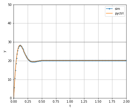
P制御

垂直駆動アームのモデルに対して、制御を行っていく

import matplotlib.pyplot as plt
import numpy as np
import pandas as pd
import control.matlab as pyctrl

g  = 9.81                # 重力加速度[m/s^2]
l  = 0.2                 # アームの長さ[m]
M  = 0.5                 # アームの質量[kg]
mu = 1.5e-2              # 粘性摩擦係数[kg*m^2/s]
J  = 1.0e-2              # 慣性モーメント[kg*m^2]

target = 30 # 目標角度 [deg]
kp = 2.0

ステップ応答

下記のスクリプトで数値シミュレーションを行う

dt = 0.0001

t_s = [0.0]
x_s = [0.0]
v_s = [0.0]
a_s = [0.0]
F_s = [0.0]
ref_s = [0.0]

for i in range(20000):
    ref = target
    ref_s += [ref]
    F_s += [(ref - x_s[-1]) * kp]
    a_s += [(- mu * v_s[-1] - M * g * l * x_s[-1] + F_s[-1]) / J]
    v_s += [v_s[-1] + a_s[-1] * dt]
    x_s += [x_s[-1] + v_s[-1] * dt]
    t_s += [t_s[-1] + dt]

df = pd.DataFrame()
df['in']  = F_s[::100]
df['out'] = x_s[::100]
df.index  = t_s[::100]

結果をプロットし、controlモジュールの結果と比較する

fig = plt.figure(figsize=(6, 5))
ax1 = fig.add_subplot(1, 1, 1)

ax1.plot(df.index, df['out'], '.-', label='sim')

# controlモジュールによるステップ応答と比較
P = pyctrl.tf([0, 1], [J, mu, M *g *l])
K = pyctrl.tf([0, kp], [0, 1])
Gyr = pyctrl.feedback(P * K, 1)
y,t = pyctrl.step(Gyr, np.arange(0, 2, 0.01))
ax1.plot(t, y*target, '-', label='pyctrl')

ax1.axhline(target, color="k", linewidth=0.5)
ax1.set_xlim(0, 2); ax1.set_ylim(0, 50)
ax1.legend(); ax1.grid()
ax1.set_ylabel('y'); ax1.set_xlabel('t')
fig.tight_layout()

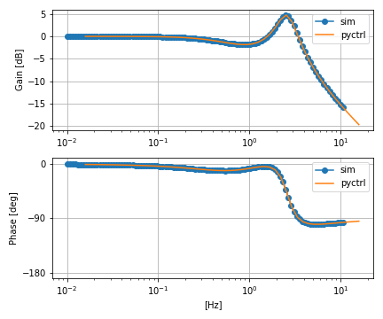
周波数特性

0.01Hz ~ 10Hz までを等比で100分割する

hz_s = []
hz = 0.01
while True:
    if hz > 10 * 10 ** (3 / 100):
        break
    hz_s.append(hz)
    hz = hz * 10 ** (3 / 100)

各周波数の正弦波を目標に入れて周波数特性を取得する

dt = 0.0001
df_list = []
for hz in hz_s:
    t_s = [0.0]
    x_s = [0.0]
    v_s = [0.0]
    a_s = [0.0]
    F_s = [0.0]
    ref_s = [0.0]

    for i in range(50000):
        ref = target * np.sin(2.0 * np.pi * hz * t_s[-1])
        ref_s += [ref]
        F_s += [(ref - x_s[-1]) * kp]
        a_s += [(- mu * v_s[-1] - M * g * l * x_s[-1] + F_s[-1]) / J]
        v_s += [v_s[-1] + a_s[-1] * dt]
        x_s += [x_s[-1] + v_s[-1] * dt]
        t_s += [t_s[-1] + dt]

    df = pd.DataFrame()
    df['in']  = ref_s[30000:]
    df['out'] = x_s[30000:]
    df.index  = t_s[30000:]
    df_list += [df]

時系列波形からゲインと位相変化を取得する関数

from scipy.optimize import curve_fit

def sin_func(x, p0, p1, p2):
    return p0 * np.sin(2.0 * np.pi * p1 * x + p2)

def _convert_phase(phase):
    phase += 180
    phase %= 360
    if phase < 0:
        phase += 180
    else:
        phase -= 180
    return phase

def _convert_param(param):
    param = param.copy()
    param[2] = param[2] / np.pi * 180
    if param[0] < 0:
        param[0] = -param[0]
        param[2] += 180

    param[2] = _convert_phase(param[2])

    return param

def calc_f_func(param1, param2):
    param1 = _convert_param(param1)
    param2 = _convert_param(param2)

    freq = param1[1]
    gain = param2[0] / param1[0]
    phase = param2[2] - param1[2]
    phase = _convert_phase(phase)

    return param1, param2, freq, gain, phase

周波数解析を実施

data_s = []
for hz, df in zip(hz_s, df_list):
    p0 = [target, hz, 0.0]
    p1, conv = curve_fit(sin_func, np.array(df.index), np.array(df['in']), p0=p0)

    p0 = [target, hz, 0.0]
    p2, conv = curve_fit(sin_func, np.array(df.index), np.array(df['out']), p0=p0)

    param1, param2, freq, gain, phase = calc_f_func(p1, p2)

    data_s.append([freq, gain, phase])

df_res = pd.DataFrame(data_s)
df_res.columns = ['freq', 'gain', 'phase']

結果を表示する
これもcontrolモジュールと比較する

fig = plt.figure(figsize=(6, 5))
ax1 = fig.add_subplot(2, 1, 1)
ax2 = fig.add_subplot(2, 1, 2)

ax1.plot(df_res['freq'], np.log10(df_res['gain'])*20.0, 'o-', label='sim')
ax2.plot(df_res['freq'], df_res['phase'], 'o-', label='sim')

K = pyctrl.tf([0, kp], [0, 1])
Gyr = pyctrl.feedback(P*K, 1)
gain, phase, w = pyctrl.bode(Gyr, pyctrl.logspace(-1,2), plot=False)
ax1.plot(w/(2*np.pi), 20*np.log10(gain), label='pyctrl')
ax2.plot(w/(2*np.pi), phase*180/np.pi, label='pyctrl')

ax2.set_ylim(-190, 10); ax2.set_yticks([-180, -90, 0])
ax1.legend(); ax1.grid(); ax1.set_xscale('log')
ax1.set_ylabel('Gain [dB]')
ax2.legend(); ax2.grid(); ax2.set_xscale('log')
ax2.set_xlabel('[Hz]')
ax2.set_ylabel('Phase [deg]')
fig.tight_layout()

PD制御

D制御を加えることで、振動を抑えることができる

kp = 2
kd = 0.2

ステップ応答

目標値と現在値の差分（偏差）を演算し、
前回の偏差との差分からD成分を算出する

dt = 0.0001

t_s = [0.0]
x_s = [0.0]
v_s = [0.0]
a_s = [0.0]
F_s = [0.0]
ref_s = [0.0]
pre_err = 0.0

for i in range(20000):
    ref = target
    ref_s += [ref]
    err = ref - x_s[-1]
    F_s += [ err * kp + (err - pre_err) * kd / dt]
    a_s += [(- mu * v_s[-1] - M * g * l * x_s[-1] + F_s[-1]) / J]
    v_s += [v_s[-1] + a_s[-1] * dt]
    x_s += [x_s[-1] + v_s[-1] * dt]
    t_s += [t_s[-1] + dt]
    pre_err = err

df = pd.DataFrame()
df['in']  = F_s[::100]
df['out'] = x_s[::100]
df.index  = t_s[::100]

fig = plt.figure(figsize=(6, 5))
ax1 = fig.add_subplot(1, 1, 1)

ax1.plot(df.index, df['out'], '.-', label='sim')

# controlモジュールによるステップ応答と比較
P = pyctrl.tf([0, 1], [J, mu, M *g *l])
K = pyctrl.tf([kd, kp], [0, 1])
Gyr = pyctrl.feedback(P * K, 1)
y,t = pyctrl.step(Gyr, np.arange(0, 2, 0.01))
ax1.plot(t, y*target, '-', label='pyctrl')

ax1.axhline(target, color="k", linewidth=0.5)
ax1.set_xlim(0, 2); ax1.set_ylim(0, 50)
ax1.legend(); ax1.grid()
ax1.set_ylabel('y'); ax1.set_xlabel('t')
fig.tight_layout()

周波数特性

dt = 0.0001
df_list = []
for hz in hz_s:
    t_s = [0.0]
    x_s = [0.0]
    v_s = [0.0]
    a_s = [0.0]
    F_s = [0.0]
    ref_s = [0.0]
    pre_err = 0.0

    for i in range(50000):
        ref = target * np.sin(2.0 * np.pi * hz * t_s[-1])
        ref_s += [ref]
        err = ref - x_s[-1]
        F_s += [ err * kp + (err - pre_err) * kd / dt]
        a_s += [(- mu * v_s[-1] - M * g * l * x_s[-1] + F_s[-1]) / J]
        v_s += [v_s[-1] + a_s[-1] * dt]
        x_s += [x_s[-1] + v_s[-1] * dt]
        t_s += [t_s[-1] + dt]
        pre_err = err

    df = pd.DataFrame()
    df['in']  = ref_s[30000:]
    df['out'] = x_s[30000:]
    df.index  = t_s[30000:]
    df_list += [df]

data_s = []
for hz, df in zip(hz_s, df_list):
    p0 = [target, hz, 0.0]
    p1, conv = curve_fit(sin_func, np.array(df.index), np.array(df['in']), p0=p0)

    p0 = [target, hz, 0.0]
    p2, conv = curve_fit(sin_func, np.array(df.index), np.array(df['out']), p0=p0)

    param1, param2, freq, gain, phase = calc_f_func(p1, p2)

    data_s.append([freq, gain, phase])

df_res = pd.DataFrame(data_s)
df_res.columns = ['freq', 'gain', 'phase']

fig = plt.figure(figsize=(6, 5))
ax1 = fig.add_subplot(2, 1, 1)
ax2 = fig.add_subplot(2, 1, 2)

ax1.plot(df_res['freq'], np.log10(df_res['gain'])*20.0, 'o-', label='sim')
ax2.plot(df_res['freq'], df_res['phase'], 'o-', label='sim')

K = pyctrl.tf([kd, kp], [0, 1])
Gyr = pyctrl.feedback(P*K, 1)
gain, phase, w = pyctrl.bode(Gyr, pyctrl.logspace(-1,2), plot=False)
ax1.plot(w/(2*np.pi), 20*np.log10(gain), label='pyctrl')
ax2.plot(w/(2*np.pi), phase*180/np.pi, label='pyctrl')

ax2.set_ylim(-190, 10); ax2.set_yticks([-180, -90, 0])
ax1.legend(); ax1.grid(); ax1.set_xscale('log')
ax1.set_ylabel('Gain [dB]')
ax2.legend(); ax2.grid(); ax2.set_xscale('log')
ax2.set_xlabel('[Hz]')
ax2.set_ylabel('Phase [deg]')
fig.tight_layout()

D制御で、ピークゲインが抑えられ、振動が小さくなる

PID制御

I制御を加えて、定常偏差を押さえる

kp = 2
kd = 0.1
ki = 10

ステップ応答

偏差を積算し、I成分として使用する

dt = 0.0001

t_s = [0.0]
x_s = [0.0]
v_s = [0.0]
a_s = [0.0]
F_s = [0.0]
ref_s = [0.0]
pre_err = 0.0
integ = 0.0

for i in range(20000):
    ref = target
    ref_s += [ref]
    err = ref - x_s[-1]
    integ += err
    F_s += [ err * kp + (err - pre_err) * kd / dt + integ * ki * dt]
    a_s += [(- mu * v_s[-1] - M * g * l * x_s[-1] + F_s[-1]) / J]
    v_s += [v_s[-1] + a_s[-1] * dt]
    x_s += [x_s[-1] + v_s[-1] * dt]
    t_s += [t_s[-1] + dt]
    pre_err = err

df = pd.DataFrame()
df['in']  = F_s[::100]
df['out'] = x_s[::100]
df.index  = t_s[::100]

fig = plt.figure(figsize=(6, 5))
ax1 = fig.add_subplot(1, 1, 1)

ax1.plot(df.index, df['out'], '.-', label='sim')

# controlモジュールによるステップ応答と比較
P = pyctrl.tf([0, 1], [J, mu, M *g *l])
K = pyctrl.tf([kd, kp, ki], [1, 0])
Gyr = pyctrl.feedback(P * K, 1)
y,t = pyctrl.step(Gyr, np.arange(0, 2, 0.01))
ax1.plot(t, y*target, '-', label='pyctrl')

ax1.axhline(target, color="k", linewidth=0.5)
ax1.set_xlim(0, 2); ax1.set_ylim(0, 50)
ax1.legend(); ax1.grid()
ax1.set_ylabel('y'); ax1.set_xlabel('t')
fig.tight_layout()

周波数特性

dt = 0.0001
df_list = []
for hz in hz_s:
    t_s = [0.0]
    x_s = [0.0]
    v_s = [0.0]
    a_s = [0.0]
    F_s = [0.0]
    ref_s = [0.0]
    pre_err = 0.0
    integ = 0.0

    for i in range(50000):
        ref = target * np.sin(2.0 * np.pi * hz * t_s[-1])
        ref_s += [ref]
        err = ref - x_s[-1]
        integ += err
        F_s += [ err * kp + (err - pre_err) * kd / dt + integ * ki * dt]
        a_s += [(- mu * v_s[-1] - M * g * l * x_s[-1] + F_s[-1]) / J]
        v_s += [v_s[-1] + a_s[-1] * dt]
        x_s += [x_s[-1] + v_s[-1] * dt]
        t_s += [t_s[-1] + dt]
        pre_err = err

    df = pd.DataFrame()
    df['in']  = ref_s[30000:]
    df['out'] = x_s[30000:]
    df.index  = t_s[30000:]
    df_list += [df]

data_s = []
for hz, df in zip(hz_s, df_list):
    p0 = [target, hz, 0.0]
    p1, conv = curve_fit(sin_func, np.array(df.index), np.array(df['in']), p0=p0)

    p0 = [target, hz, 0.0]
    p2, conv = curve_fit(sin_func, np.array(df.index), np.array(df['out']), p0=p0)

    param1, param2, freq, gain, phase = calc_f_func(p1, p2)

    data_s.append([freq, gain, phase])

df_res = pd.DataFrame(data_s)
df_res.columns = ['freq', 'gain', 'phase']

fig = plt.figure(figsize=(6, 5))
ax1 = fig.add_subplot(2, 1, 1)
ax2 = fig.add_subplot(2, 1, 2)

ax1.plot(df_res['freq'], np.log10(df_res['gain'])*20.0, 'o-', label='sim')
ax2.plot(df_res['freq'], df_res['phase'], 'o-', label='sim')

K = pyctrl.tf([kd, kp, ki], [1, 0])
Gyr = pyctrl.feedback(P*K, 1)
gain, phase, w = pyctrl.bode(Gyr, pyctrl.logspace(-1,2), plot=False)
ax1.plot(w/(2*np.pi), 20*np.log10(gain), label='pyctrl')
ax2.plot(w/(2*np.pi), phase*180/np.pi, label='pyctrl')

ax2.set_ylim(-190, 10); ax2.set_yticks([-180, -90, 0])
ax1.legend(); ax1.grid(); ax1.set_xscale('log')
ax1.set_ylabel('Gain [dB]')
ax2.legend(); ax2.grid(); ax2.set_xscale('log')
ax2.set_xlabel('[Hz]')
ax2.set_ylabel('Phase [deg]')
fig.tight_layout()